Introduction to `{gardenr}`

Example

Here is an example of using cross_validate_it() to help with hyperparameter tuning.

#devtools::install_github("Chhr1s/gardenr")
library(gardenr)
library(glmertree)
library(dplyr)

Simulate some data

Here’s a function within the package to simulate some multilevel data. It has defaults, but these can be changed. use ?sim_multilevel() for details. I made the standard deviation of residual variance large in the example at both level 1 and level 2 to make the difference between default hyperparameters and tuned models more dramatic.

dat <- sim_multilevel(residual_var_sd_1 = 2, residual_var_sd_2 = 6)

Split Data & Make CV Object

Wherever possible, I wanted to rely on good functions from the tidymodels framework. We can use rsample to spit the data and make a cross-validation object.

example_split <- rsample::initial_split(dat)
example_train <- rsample::training(example_split)
example_test  <-  rsample::testing(example_split)
cv <- rsample::vfold_cv(data = example_train, v = 10)

Make a `Formula` object

This is the proposed GLMM tree formula. This is not a normal formula object, but a Formula object instead. See ?Formula::as.Formula for an explanation of the differences.

ex_formula <-
   Formula::as.Formula(
      'outcome ~ small_1 |
      (1 | id_vector) |
      small_2 + small_c_1 + small_c_2 + nuisance_1a + nuisance_c_1a'
      )

Make a Tuning Grid

We can then use dials to make a tuning grid. Notice that the parameter objects for GLMM trees have already been made and are in gardenr (e.g., alpha_par())

tuning_grid <-
  dials::grid_max_entropy(
    maxdepth_par(maxdepth_min = 2L, maxdepth_max = 20L),
    alpha_par(alpha_min = 0.10, alpha_max = 0.001),
    trim_par(trim_min = 0.01, trim_max = 0.5),
    size = 10
  )
tuning_grid
#> # A tibble: 10 × 3
#>    maxdepth_par alpha_par trim_par
#>           <int>     <dbl>    <dbl>
#>  1           13   0.0996    0.402 
#>  2           19   0.0548    0.0993
#>  3           14   0.00564   0.0229
#>  4           10   0.0447    0.158 
#>  5           19   0.00537   0.273 
#>  6           11   0.0116    0.453 
#>  7           15   0.0476    0.334 
#>  8            2   0.0664    0.471 
#>  9           12   0.0811    0.0343
#> 10            3   0.0837    0.0433

Fit the Model to the Cross-Validated Data

Here we fit the model to the cross-validated object.

fitted <-
   cross_validate_it(
      cv_obj = cv,
      seed = 713,
      tuning_grid = tuning_grid,
      mod_formula = ex_formula, 
      cluster = id_vector
      )

See Best Fitting Hyperparameters

best_fit <- 
  fitted %>% 
  arrange(mean_rmse) 
best_fit
#> # A tibble: 10 × 8
#>    grid_index maxdepth_par alpha_par trim_par mean_rmse se_rmse mean_mae  se_mae
#>         <int>        <int>     <dbl>    <dbl>     <dbl>   <dbl>    <dbl>   <dbl>
#>  1         10            3   0.0837    0.0433      2.05  0.0352   0.0125 1.80e-4
#>  2          6           11   0.0116    0.453       2.05  0.0350   0.0124 1.90e-4
#>  3          8            2   0.0664    0.471       2.05  0.0365   0.0125 1.97e-4
#>  4          5           19   0.00537   0.273       2.06  0.0366   0.0125 2.03e-4
#>  5          3           14   0.00564   0.0229      2.07  0.0358   0.0125 1.96e-4
#>  6          4           10   0.0447    0.158       2.07  0.0344   0.0125 1.85e-4
#>  7          2           19   0.0548    0.0993      2.07  0.0328   0.0126 1.76e-4
#>  8          7           15   0.0476    0.334       2.07  0.0367   0.0125 1.99e-4
#>  9          1           13   0.0996    0.402       2.08  0.0356   0.0126 1.93e-4
#> 10          9           12   0.0811    0.0343      2.08  0.0336   0.0126 1.86e-4

best_fit_trained <- 
  lmertree(
    data = example_train, 
    formula = 
      ex_formula, 
    maxdepth = best_fit$maxdepth_par[1], 
    alpha = best_fit$alpha_par[1],
    trim = best_fit$trim_par[1], 
    cluster = id_vector,
    verbose = TRUE
  )
#> 'log Lik.' -3015.466 (df=4)
#> 'log Lik.' -3011.777 (df=10)
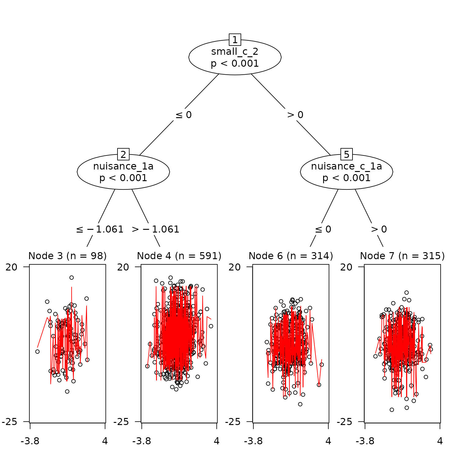
#> 'log Lik.' -3011.777 (df=10)

See Splits as Plot

plot(
  best_fit_trained, 
  which = 'tree',
  )

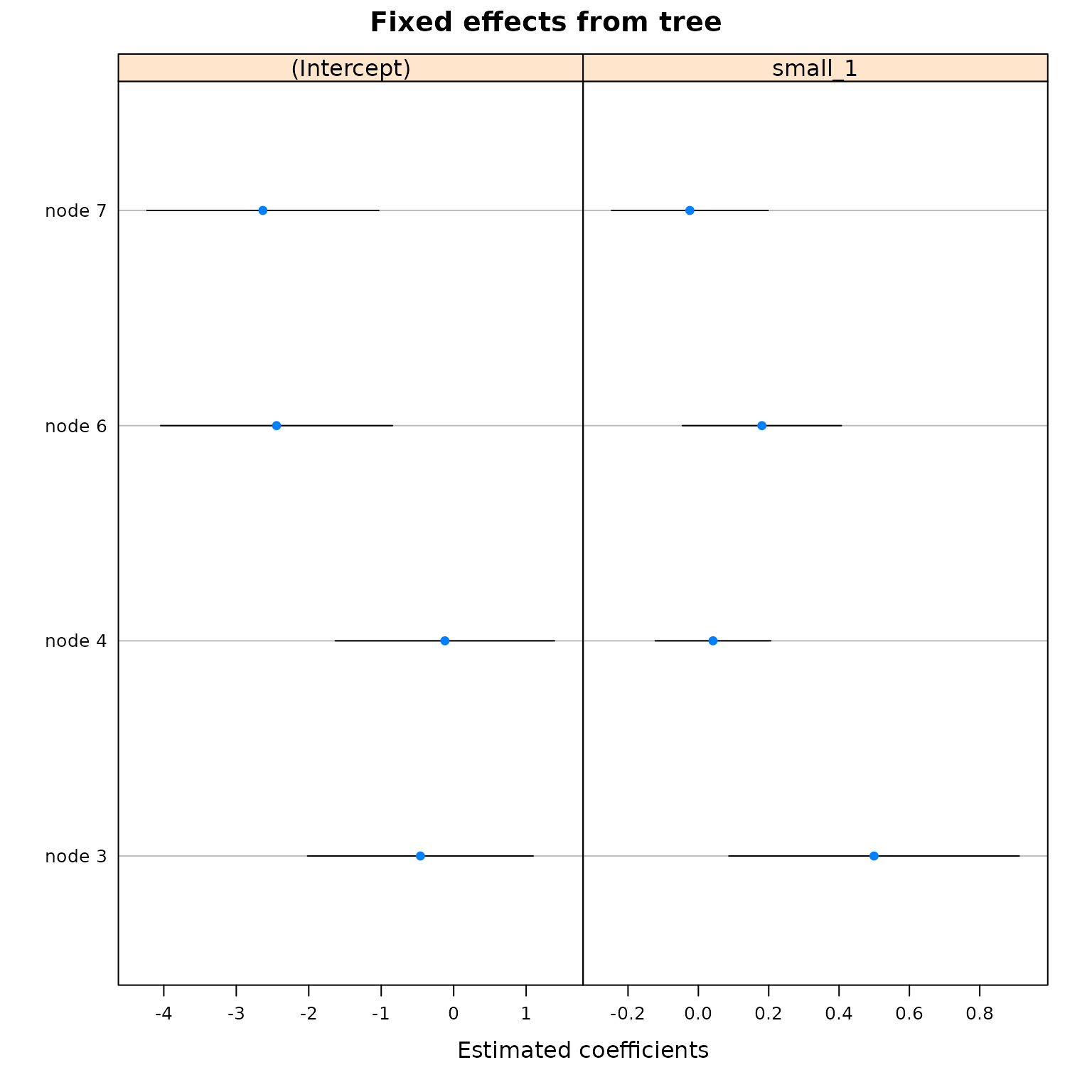
plot(
  best_fit_trained, 
  which = 'tree.coef',
  )

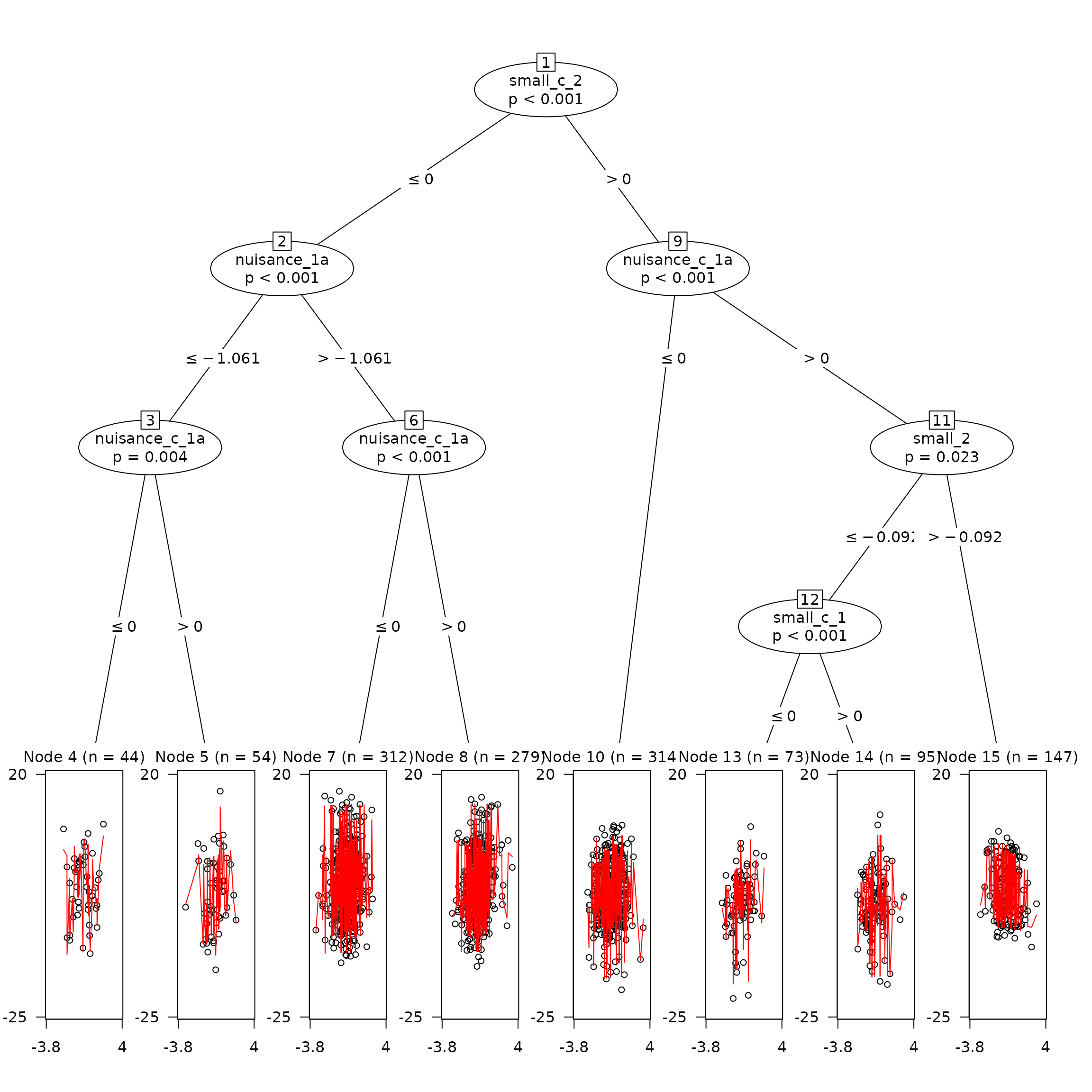
Compare this to a tree with default hyperparameters

It’s clear that this tree has made many more splits than the trained model.

untrained <- 
  lmertree(
    data = example_train, 
    formula = 
      ex_formula, 
    cluster = id_vector,
    verbose = TRUE
  )
#> 'log Lik.' -3015.466 (df=4)
#> 'log Lik.' -3009.867 (df=16)
#> 'log Lik.' -3004.441 (df=18)
#> 'log Lik.' -3003.055 (df=18)
#> 'log Lik.' -3004.441 (df=18)
#> 'log Lik.' -3003.055 (df=18)

plot(
  untrained,  
  which = 'tree'
  )

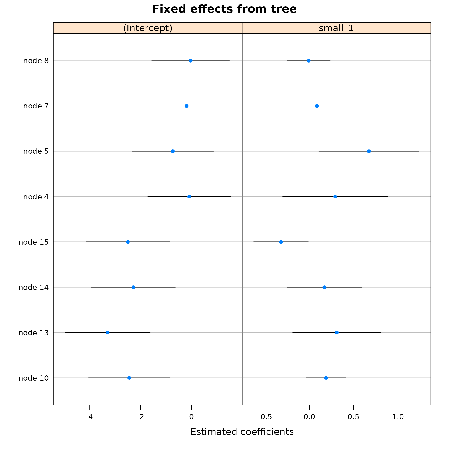
plot(
  untrained, 
  which = 'tree.coef',
  )

Get RMSE for unseen data

We see here that the model fits unseen data slightly better than the model with default hyperparameters.

example_test %>% 
  mutate(
    predictions_tuned =
      predict(
        best_fit_trained, 
        newdata = ., 
        allow.new.levels = TRUE
        ),
    predictions_default_hyperparams =
      predict(
        untrained, 
        newdata = ., 
        allow.new.levels = TRUE
        ),
    ) %>% 
  summarize(
    tuned_RMSE = 
      rmse(observed_y = outcome, predicted_y = predictions_tuned),
    default_hyperparams_RMSE = 
      rmse(observed_y = outcome, predicted_y = predictions_default_hyperparams)
    )
#>   tuned_RMSE default_hyperparams_RMSE
#> 1   2.020963                 2.044691

Introduction to {gardenr}